SECURITY BREACH? CALL 888.234.5990 EXT 9999

Overcome Imbalance in your datasets — PART II

In PART I of this article, we discussed the implications of imbalance in datasets and how it affects the accuracy of prediction of minority classes. After going over some techniques and implications, we can now move on to drawing lessons and conclusions.

Before analyzing the results, let’s set the ground rules:

  • Main dataset was split into Train & Test in a 80–20 ratio.
  • The Train Dataset was oversampled using SMOTE, KMeans SMOTE, SVM SMOTE and SMOTE ENN (Oversample minority + Undersample majority). Separate datasets were created for each.
  • Separate models were trained with each dataset.
  • XGBoost was selected due to its high performance as a binary classifier for tabular data.
  • AWS Built-In XGBoost was used in a AWS SageMaker environment.
  • To even conditions, a Hyper-Parameter tuning job was performed for each model. Best Hyper-Parameters were selected for each training job.
  • Results were analyzed using a confusion matrix. Emphasizing in the false-negatives, as it’s the most critical condition.
      Having stated these ground rules, let’s take a look at our results:

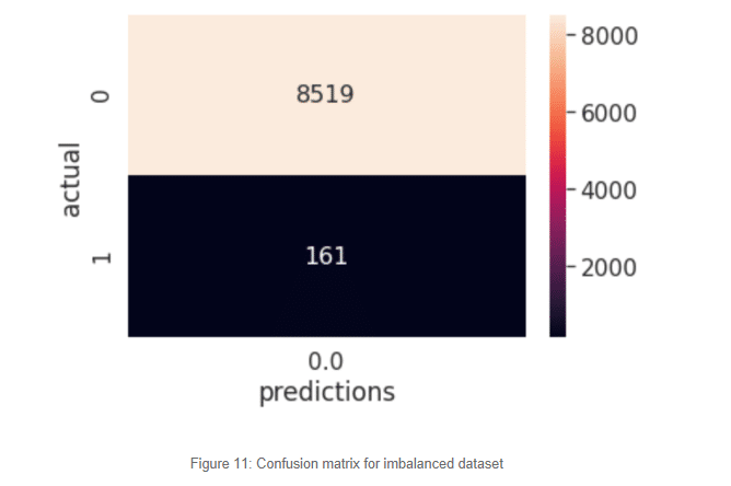
Model Training with Raw Dataset

Something quite interesting is happening here. The class distribution is so skewed that our model has learned that the best way to classify our target variable is to predict everything as a negative case. Of course, it has seen over 30 thousand negative cases and just over eight hundred positive cases. At this point it’s almost like a random guess, the algorithm determines the best way to classify the never-seen-before examples is to mark them all as zeroes. This is exactly the problem we face with imbalance datasets. Those 161 cases predicted as healthy are most likely to develop a stroke and our model was not able to predict it. The cost of misclassification at this scale is impossible to intolerable.

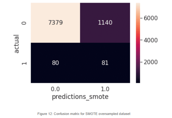
Model Training with SMOTE resampled dataset

Now this looks a lot different than the earlier model. When increasing the minority class artificially, the model can make a better generalization. We can now predict almost half of the positive cases, which is an improvement. Still, there are a lot of misclassifications in the negative cases. There are a lot of negative cases that are being marked as possible stroke victims, but for our most sensitive cases, which are the actual positives, we can see that our classifier is doing a much better job.

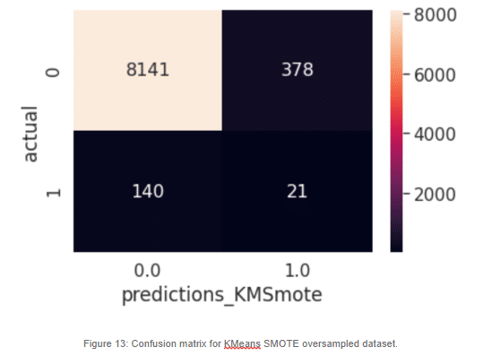
Model Training with KMeans-SMOTE resampled dataset

For our KMeans SMOTE variant, we can see that it performs worse than regular SMOTE. We can see a degradation of the false negatives. In this case, without further investigation, we cannot make a solid statement on why KMeans SMOTE is the lowest performer, but it may have to do with the fact that KMeans itself has its own critical Hyper-Parameter, k, which should be optimized. If a sub-optimal number of clusters is generated, perhaps our artificial samples won’t help our model. Supplemental tuning of the KMeans SMOTE and the model itself may help improve the performance of the classifier, however we will not address this in this article.

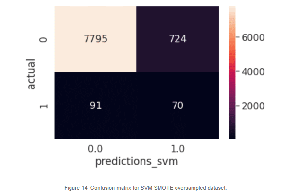
Model Training with SVM-SMOTE resampled dataset

SVM-SMOTE resampled dataset produces a better result than the KMeans SMOTE variant when it comes to the positive cases. This could mean that the area where misclassification is happening is at the border of the two classes. We could further improve this model by tweaking the class distribution under sampling the majority class.

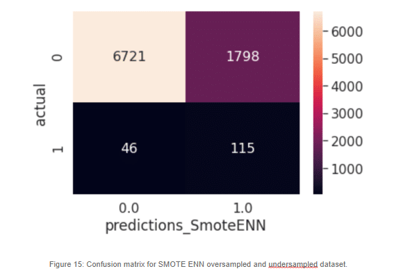
Model Training with SMOTE resampled and undersampled dataset

Lastly, we trained a classification model using both SMOTE oversampling for increasing the minority class and decreasing the majority class. Of the models described, this one produces the better results regarding the false negatives. Still there is a lot of misclassifications in the actual negatives, but for our most important cases, this model achieves better performance than its peers.

Conclusions and Contributions

The dataset we just worked with represents a sensitive case. It is a medical condition that may be a life-or-death situation. For this reason our model should be extremely good at predicting the possible stroke victims.

This is an example where our false negatives are intolerable, and we need to reduce them the best way we can.

Working with the imbalanced dataset showed us that our model is rather useless: it fails to predict the stroke cases.

When we successfully overcame the imbalance of the dataset our models started to predict those possible victims of stroke. Depending on the technique used, the response of the model was better or worse, but at the end of the day, solving the imbalance is the first step to building an effective classification model.

Strokes, as with other medical conditions, are perfect examples of imbalanced datasets. And though the use of AI should be considered as a complementary approach to human expertise, solving critical and inherent problems such as the class imbalance, will make technologies like AI and ML much better suited to address important problems we face today.

Please refer to our Repository where you can find the Notebooks with the complete code for this solution.

What about AWS Services for overcoming the Imbalance in our datasets?

When working with Machine Learning in AWS, SageMaker is the go-to place to deploy our ML workloads.

AWS introduced Amazon SageMaker DataWrangler as a new capability for data scientists to prepare datasets for machine learning applications using graphical interfaces.

AWS Sagemaker DataWrangler now provides a Balance feature that makes it very easy to implement Random Undersample, Random Oversample and SMOTE, without the need for working the code or doing other time-consuming tasks.

Now that we understand the true nature of working with imbalanced datasets, making the shift to a managed service such as AWS Sagemaker DataWrangler should be a smooth transition.

So, if you want to know more about AWS Sagemaker, DataWrangler or any other ML theme; don’t hesitate to contact us and we will be happy to help.

Appendix

The following section is a complement to the article and provides a comprehensive overview of the procedures to implement the Oversampling Techniques described in the article.

We will address the installation of required libraries, we will also provide code resources for creating artificial datasets using Scikit-Learn, force its imbalance using make_imbalance and from there implement our oversampling techniques.

We also provide a visual representation of each oversampling technique, that may be useful when understanding similarities and differences.

Similarly to the article, the notebook for this section is also available in the repository.

Imbalanced-Learn command reference

For the following section, we will discuss the different methods available for the different oversampling techniques discussed in previous chapters. We will focus on Imbalanced-Learn, an open source library relying on scikit-learn which provides tools to deal with classification with imbalanced datasets

Imbalance-Learn Library installation & Basic usage

The easiest way to install Imbalanced-Learn library is via PyPi’s repositories, from where we can install it via pip<

pip install -U imbalanced-learn

The package is also available in Anaconda Cloud and from source on GitHub. Imbalance-Learn adds sampling functionality. To resample a dataset each sampler implements:

data_resampled, targets_resampled = obj.fit_resample(data, targets)

The same structure will apply for our oversamplers, where data represents our dataset and can be a numpy array or a pandas dataframe. For the target, the input should be a one-dimensional numpy array or pandas series.

As for the output, our oversample will return a data_resampled dataset and a target resamped series.

We will see that no matter which SMOTE variant we require, the procedure to invoke the methods and the outputs will be almost the same. Now, let’s explore the different methods that Imbalanced-Learn offers to implement the previously discussed oversampling techniques. We will generate dummy imbalanced datasets and from there, call the different methods to rebalance. Let’s take a look at how we generate the datasets first.

Creating an artificial Imbalanced Dataset

Scikit-Learn includes various random sample generators that can be used to build artificial datasets of controlled size and complexity.

We will leverage this technique to generate our dummy datasets, and then make it purposely imbalanced using the make_imbalance method.

from sklearn.datasets import make_moons
# Use Make moons to generate two interleaving half circles. This will generate a dataset and its labels
X, y = make_moons(n_samples = 5000, shuffle = True, noise = 0.5 , random_state = 42)
# Transform numpy series generated by Make Moons into Pandas Dataframe to better handling
X = pd.DataFrame (data = X, columns= [“feature1”, “feature2”])
y = pd.DataFrame (data = y)

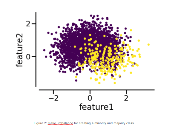
Snippet of code XXX shows us how to generate a random dataset for binary classification. Make_moons, according to official documentation from scikit-learn, “generates bidimensional binary classification datasets that are challenging to certain algorithms. In our case we choose to generate a 5000 samples dataset. In order to take a closer look at it, we will rely on matplotlib to graph this dataset to better understand data distribution.

# Lets graph 
ax = X.plot.scatter( 
x=”feature1″, 
y=”feature2″, 
c=y, 
colormap=”viridis”, 
colorbar=False, 
) 
sns.despine(ax=ax, offset=10)

The output of this scatter plot is displayed as follows: 

Figure ZZZ shows us the recently created dataset. Now, let’s go ahead and create an imbalance. 

# Now, use Make_imbalance to create an imbalanced dataset. We use a 90–10 distribution 
X_resampled, y_resampled = make_imbalance (X, y, sampling_strategy = {0:2500, 1:250}, multiplier = 0.1, minority_class = 1)
 

Code snippet XYZ is about forcing an imbalance in our dataset. As you can see, what we did here is create a ratio of roughly 90–10 between classes. Originally, our dataset was perfectly balanced, with a 50–50 distribution (2500 samples for each class), now what we did is to undersize one class to create the skewed distribution. 

Using the same code as before (referencing the new resampled dataset), let’s graph again: 

Now that we have an imbalanced distribution, it’s time for splitting our data. 

A very important note here: No matter which technique you use to overcome an Imbalanced Dataset, you must always apply it after partitioning your data in train-test. 

If you oversample, do it on the training dataset, never on the validation dataset. Why? Well, because if we oversample on the validation dataset we will “contaminate” our model evaluation phase with data that will not reflect our reality. Remember, our objective is to build models that generalize over the observations and in the real world, for this kind of problems, it is normal that the minority class is underrepresented and appears in few cases and what we really need is to correctly predict these minority observations. 

Having said this, let’s take a look at the way we partition our dataset: 

# Split into train-test 
from sklearn.model_selection import train_test_split 
X_train, X_test, y_train, y_test = train_test_split(X_resampled, y_resampled, test_size = .3, random_state=42) 

Train_Test_Split is a great way to split our datasets. Is a method of Scikit-Learn and its main advantage is that it will not only split our dataset, but it will do a random shuffle too, that will ensure that our dataset is properly randomized and then split. Not shuffling the data before splitting may cause an abnormal proportion between classes in training and validation datasets, so it’s nice to have randomization and splitting together. In our example we define a validation size of 0.3, which means 30% validation and 70% training. This is usually the best practice. 

Now that we have our imbalance dataset split into training and testing, it’s time to make use of our resamplers. We will demonstrate default SMOTE, KMeans SMOTE and SVM SMOTE. 

Default SMOTE

# Import SMOTE from imblearn 
from imblearn.over_sampling import SMOTE 
sm = SMOTE (sampling_strategy = “not majority” , random_state = 42)# Resample dataset  
X_train_oversampled, y_train_oversampled = sm.fit_resample(X_train, y_train) 

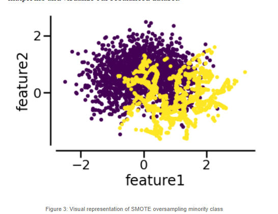
As described at the beginning of this section, the use of the oversamplers is almost identical disregarding which we use. We define a dataset_resampled , labels_resampled pair as outputs and call our resampler object created earlier with our imbalance train dataset and train labels as inputs. We will use the same snippet of code to call matplotlib and visualize our rebalanced dataset. 

Remember that in its plain form, SMOTE will randomly generate samples in the segments connecting the K Nearest adjacent minority class instances and will repeat this process until the dataset is no longer imbalanced. But sometimes we want to place synthetic samples with a different approach. We will now show you how to implement KMeans and SVM Smote, which relies on an unsupervised algorithm to determine where to place the synthetic samples in a more efficient way.

K-Means SMOTE

To properly demonstrate the following methods, we proceed to create a new artificial dataset, specially created for binary classification, using the make_blobs method. According to the official documentation, make_blobs is a method for generating isotropic Gaussian blobs, which are perfect for clustering purposes, and this is how we applied it: 

# Use make_blobs to create dataset 
from sklearn.datasets import make_blobs 
X, y = make_blobs (n_samples = 500, centers = 2, n_features = 2, cluster_std = 3, center_box = (-7.0,7.0) , random_state = 42)# Convert to pandas dataframe for better handling 
import pandas as pd 
X = pd.DataFrame (data = X, columns= [“feature1”, “feature2”]) 
y = pd.DataFrame (data = y)# Use make_imbalance to create a skewed dataset 
from imblearn.datasets import make_imbalance 
X_resampled, y_resampled = make_imbalance (X, y, sampling_strategy = {0:250, 1:50}, multiplier = 0.1, minority_class = 1)# Split in train-test 
from sklearn.model_selection import train_test_split 
X_train, X_test, y_train, y_test = train_test_split(X_resampled, y_resampled, test_size = .3, random_state=42) 

Now, we are ready to apply our resampling techniques: SVM SMOTE and K-Means SMOTE. 

from imblearn.over_sampling import KMeansSMOTE 
sm = KMeansSMOTE(random_state=42) 
X_over, y_overs = sm.fit_resample(X_train, y_train) 

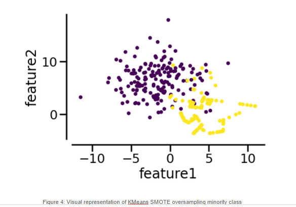
Previous snippet shows the use of KMeans SMOTE for synthetic sample generation. As you can see it follows the same structure. As result we get the following output: 
KMeans SMOTE first create clusters to determine which areas are a better fit for sample generation. Data density in outer regions may be a consequence of this clustering step.

SVM SMOTE

from imblearn.over_sampling import SVMSMOTE 
sm = SVMSMOTE(random_state=42) 
X_res_svm, y_res_svm = sm.fit_resample(X_train, y_train) 

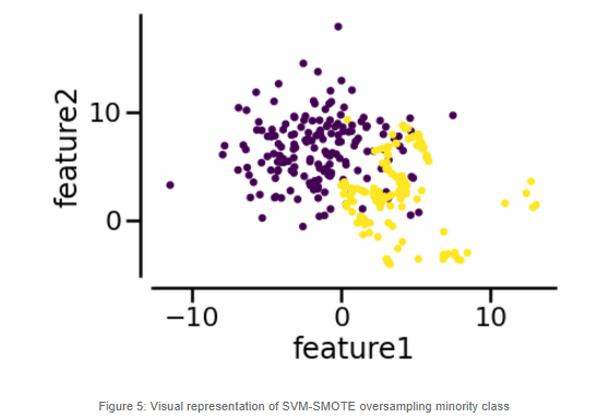
Same general principle for calling the method. Now let’s take a look at the output: 

With the same dataset we can see that synthetic sample positioning is totally different from what we got from KMeans SMOTE. In this case, the SVM clustering step enables us create a bigger sample density in the class boundary

As shown in the previous paragraphs, the implementation of the resamplers is a very simplistic process thanks to the implementation of open source libraries. Independent of the resamplerof our choice, applying such techniques to our code is similar among them and proves to be an easy setup for addressing the imbalance. Of course, the result will vary, and there is not a single silver bullet that will solve every problem. Once we rebalance our dataset, we still have to train and evaluate our classifier and we may get better or worse results depending on the approach we chose. In the next section we will test different SMOTE variants and see the impact of the classifier’s effectiveness.