Overcome Imbalance in your Datasets — PART I
A dataset is imbalanced when the classes are not approximately equally distributed. This means that there is a severe skew in the class representation. So, how severe can this skewness be? Well, there are studies that show imbalances on the order of 100 to 1 in fraud detection, as well as imbalances up to 100,000 to 1 in other applications. This kind of use case, where there are very few samples of a class relative to others, maybe seen as finding a needle in a haystack problem.
Let’s dive a little further into this. Imagine we have a dataset where classes appear in a 999:1 ratio. The algorithm is clever, it has mostly seen one type of case, therefore the classifier will try to predict every example as if it belongs to the majority class. And by doing so, we would have 99% accuracy in our model. This is a tough benchmark to beat, even for an algorithm. However, and no matter how high our accuracy is, this approach has bigger problems to address.
First of all, it assumes equal error costs. This means that the error of misclassifying an observation has the same consequences regardless of the class.
In the real world, things are different. Classification often leads to action, and actions have an effect. In cases where the prediction of the minority class is most important, having a random guess approach is simply not tolerable. Because misclassifying the minority class may have consequences such as allowing a fraudulent transaction, ignoring a malfunctioning part, and not detecting a disease. For example, a typical mammography dataset might contain 98% normal pixels and 2% abnormal pixels. The nature of this kind of application requires a very high rate of detection in the minority class and allows for a small error rate in the majority class.
The consequences of misclassification may be severe, and performing the incorrect actions may be quite costly. On very rare occasions, the costs of mistakes are equivalent. In fact, it’s hard to think about a domain where the classification is indifferent to whether it makes Type 1 (False Positive) or Type 2 (False Negative) errors.
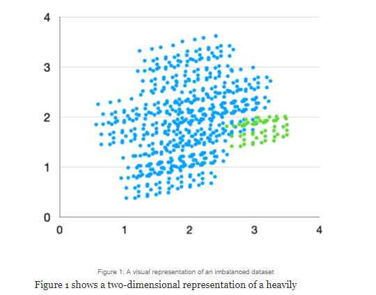
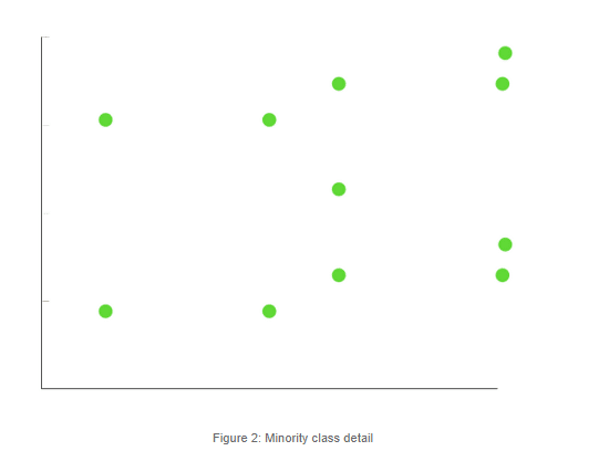
Figure 1 shows a two-dimensional representation of a heavily imbalanced dataset. As we can see, the green class is underrepresented relative to the blue class. We will show how SMOTE would work its oversampling magic. In order to show this, first, let’s zoom in a little in the green class to have a better view.
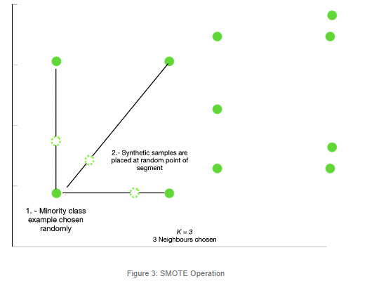
Alright, so we now have a zoomed-in picture of a portion of the green, minority class. What will happen now is that SMOTE will first select a minority class instance at random and find its K nearest minority class neighbors. Then, it will choose one of the K nearest neighbors at random and connect both to form a line segment in the feature space. The synthetic instance will be created at a random point of the segment.
As described earlier, apart from the default SMOTE behavior, described in previous paragraphs, there are other oversampling techniques based on SMOTE that may enhance our oversampling outcome. Let’s dive a little deeper into those.
In its default form, SMOTE works only with continuous features. When we are working with categorical data, SMOTE will create samples in a continuous space and we would end up with data that does not make any sense. For example, imagine we are trying to oversample a categorical feature such as “CustomerType” that has 4 possible attributes that we have encoded to values from 1 to 4. If we oversampled this data with SMOTE, we could end up with samples such as 1.34 or 2.5, which would not make any sense and would make distortion in our model. The premise behind SMOTE-NC is simple, we need to specify which features are categorical, and for these, it will pick the most frequent category of the nearest neighbors present during generation. SMOTE-NC expects categorical and continuous features in our dataset, if we have an all-categorical dataset, then SMOTEN will be our choice. SMOTEN follows the same premise as SMOTE-NC for creating synthetic observations but will expect an all-categorical dataset.
Support Vector Machine SMOTE (SVM-SMOTE) is an oversampling method that focuses on the minority class instances lying around the borderline between classes. Due to the fact that this area is most crucial for establishing the decision boundary, new instances will be generated in such a manner that the minority class area will be expanded toward the side of the majority class at the places where there appear few majority class instances.
The objective of the Support Vector Machine is to find the optimal hyperplane that separates the positive and negative classes with a maximum margin. The borderline area is approximated by the support vectors obtained after training a standard SVM classifier on the original dataset, and new instances will be randomly created along the lines joining each minority class support vector with a number of its nearest neighbors using interpolation or extrapolation technique, depending on the density of majority class instances around it.
When to choose SVM SMOTE over regular SMOTE will depend entirely by the prediction model targets and the business affected by it. If misclassification happens near the boundary decision, then SVN SMOTE may be better suited for our oversampling process.
In this section, we will demonstrate the working features of SMOTE and its different variants. The idea is to work with a highly imbalanced dataset where we can try different oversampling techniques discussed in the article and see how they perform.
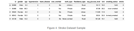
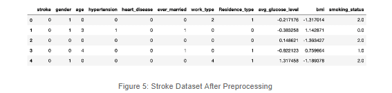
As you can see, there are features that describe some characteristics of the patients. Also, we can check out our label, stroke, which will most likely show an important skew. From this initial review, we can also verify that there are Null or Empty values, string type variables, and irrelevant columns. We will take care of those to focus on overcoming the Imbalance.
After the preprocessing stage, it’s easier for us to analyze the imbalance and try to think about a machine learning approach to develop a trustworthy model for preventing strokes.
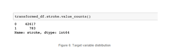
Having little knowledge about the issue we are dealing with, we can infer that of our whole sample of the population, only a few will present a stroke and, even though is the second cause of death globally, from a sample perspective, we will have a lot more negative cases than positive ones.
Roughly 2% of the whole sample has suffered a stroke. This is a case of a highly imbalanced dataset. Notice that we have less than a thousand positive cases and over 42 thousand negative cases.
We can always rely on visualization to help us understand this bias, even though in our case it’s a no-brainer.
Great, so we have the perfect dataset to demonstrate our beloved oversampling techniques.
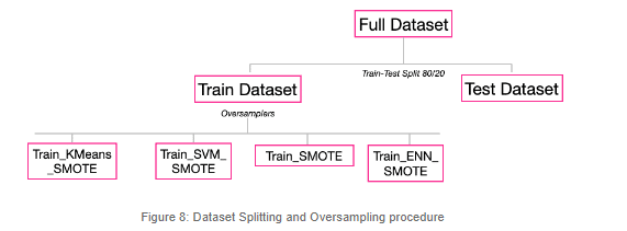
The oversampling phase is quite simple to implement thanks to libraries such as imbalance-learn; this is how we implemented the default SMOTE versions. For further references, check out the repo shared along with the article for full details.
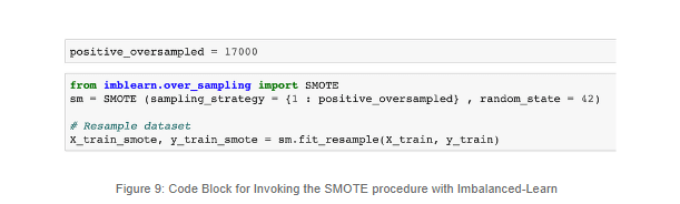
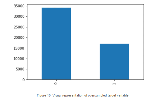
In the previous code block we can see how we are implementing SMOTE. One thing to note here is that we are not equalizing the two classes, mainly because if we do so, we will have to create over 34 thousand synthetic samples and this will definitely distort our performance. So, we will oversample, but only to a certain degree, where our minority class will reach roughly 50% of the majority class.
This is what it looks like:
We did exactly the same thing for the other SMOTE techniques to create our remaining datasets. The imbalanced-learn library makes it very simple to call different methods for every oversampling technique.